Google Data Analytics Certificate Capstone Project: Economic Growth and Fertility Rates
Executive Summary
Analysis on the relation between economic growth and fertility rates has been conducted to diagnose the falling fertility rates in the Republic of Korea. Datasets from the OECD database were analyzed through R Studio. The analysis found a correlation in GDP per capita and demystified the role of housing prices in fertility rates. The case study includes high-level recommendations to address the issue.
Scenario
I am a junior data analyst working for a think tank based in South Korea. As a member of the policy research group, I have been asked to analyze the relation between economic growth and fertility rates as the fertility rates have decreased dramatically. I have been asked to analyze economic data and fertility rates in OECD countries to gain insights and provide high-level policy recommendations.
1. Ask
1.1 Business task
Identify trends relating to economic growth and fertility rates among OECD countries and find correlations (or possible causations). Provide high-level recommendations to reverse the trend in dropping fertility rates.
Stakeholders: Hong Gil-dong (National Assembly member) and Lee Chul-soo (Senior Analyst, policy research group).
2. Prepare
2.1 Dataset used
The dataset used for this case study was sourced from data.oecd.org. The dataset has been compiled by myself and is stored on my local storage. All data is licensed under the Creative Commons Attribution 4.0 International license.
2.2 Information about the dataset
The data has been collected by the OECD from year 1950 to 2020. The data includes metrics related to population, demographics, and economic growth. The dataset includes 5 CSV files. Each document includes different quantitative data aggregated by the OECD.
| Table Name | Type | Description |
| OECD Elderly Population | CSV File | Annual elderly population data from OECD countries |
| OECD Fertility Rates | CSV File | Fertility rates data from OECD countries |
| OECD GDP | CSV File | Annual GDP from OECD countries |
| OECD Housing | CSV File | Housing price to income data from OECD countries |
| OECD Population | CSV File | Population data from OECD countries |
2.3 Data credibility and integrity
The dataset is heavily reliant on one source, however, the organization responsible for the data aggregation (OECD) is recognized as a trusted data provider of economic data due to its highly scrutinized processes. The analysis on OECD countries may invoke a sample bias when applied to developing nations since OECD nations are mostly developed economies. Additionally, the years of data collected are inconsistent since some countries have not joined the OECD until recently.
3. Process
3.1 Installing packages and opening libraries
I will be using the tidyverse package to process the dataset.
Downloading the tidyverse package.
> install.packages("tidyverse")Loading the tidyverse and tidyr package.
> library(tidyverse)
> library(tidyr)
3.2 Importing datasets
> oecd_elderly_pop <- read.csv(file = "Desktop/MyCaseStudy/OECD_ELDERLY_POPULATION.csv")
> oecd_fertility_rates <- read.csv(file = "Desktop/MyCaseStudy/OECD_FERTILITY_RATES.csv")
> oecd_gdp <- read.csv(file = "Desktop/MyCaseStudy/OECD_GDP.csv")
> oecd_housing <- read.csv(file = "Desktop/MyCaseStudy/OECD_HOUSING_PRICE_TO_INCOME.csv")
> oecd_pop <- read.csv(file = "Desktop/MyCaseStudy/OECD_POPULATION.csv")
All datasets are imported to R Studio.

3.3 Previewing and cleaning datasets
> head(oecd_elderly_pop)
> str(oecd_elderly_pop)
> head(oecd_ferility_rates)
> str(oecd_fertility_rates)
> head(oecd_gdp)
> str(oecd_gdp)
> head(oecd_housing)
> str(oecd_housing)
> head(oecd_pop)
> str(oecd_pop)
> head(worldbank_gdp_per_capita)
> str(worldbank_gdp_per_capita)
# this is an example of from the oecd_gdp data frame
> head(oecd_gdp)
LOCATION INDICATOR SUBJECT MEASURE FREQUENCY TIME Value Flag.Codes
1 AUS GDP TOT MLN_USD A 1960 25034.74
2 AUS GDP TOT MLN_USD A 1961 25326.38
3 AUS GDP TOT MLN_USD A 1962 27913.21
4 AUS GDP TOT MLN_USD A 1963 30385.72
5 AUS GDP TOT MLN_USD A 1964 32694.47
6 AUS GDP TOT MLN_USD A 1965 34489.93
> str(oecd_gdp)
'data.frame': 4829 obs. of 8 variables:
$ LOCATION : chr "AUS" "AUS" "AUS" "AUS" ...
$ INDICATOR : chr "GDP" "GDP" "GDP" "GDP" ...
$ SUBJECT : chr "TOT" "TOT" "TOT" "TOT" ...
$ MEASURE : chr "MLN_USD" "MLN_USD" "MLN_USD" "MLN_USD" ...
$ FREQUENCY : chr "A" "A" "A" "A" ...
$ TIME : int 1960 1961 1962 1963 1964 1965 1966 1967 1968 1969 ...
$ Value : num 25035 25326 27913 30386 32694 ...
$ Flag.Codes: chr "" "" "" "" ...I went further in the dataset to see if there are any other variables in each column and I found that the MEASURE column had two variables: MLN_USD and USD_CAP.

So I proceeded to count unique variables for the columns INDICATOR, SUBJECT, MEASURE, FREQUENCY.
> n_distinct(oecd_gdp$MEASURE)
[1] 2
> n_distinct(oecd_gdp$SUBJECT)
[1] 1
> n_distinct(oecd_gdp$INDICATOR)
[1] 1
> n_distinct(oecd_gdp$FREQUENCY)
[1] 1
The MEASURE column only has two variables; annual GDP and GDP per capita. So I want to separate these two metrics.
I created separate data frames for annual GDP and GDP per capita.
> oecd_gdp_annual <- filter(oecd_gdp, MEASURE == "MLN_USD")
> oecd_gdp_cap <- filter(oecd_gdp, MEASURE == "USD_CAP")
Also, I changed all the columns to lower case and more intuitive names.
> oecd_gdp_annual <- oecd_gdp_annual %>% rename(year = TIME, frequency = FREQUENCY, indicator = INDICATOR, country = LOCATION, value = Value, subject = SUBJECT, measure = MEASURE

> oecd_gdp_cap <- oecd_gdp_cap %>% rename(year = TIME, frequency = FREQUENCY, indicator = INDICATOR, country = LOCATION, value = Value, subject = SUBJECT, measure = MEASURE)
I also found that the OECD Population dataset contains two measures: total population in millions and annual population growth. Again, I will separate the two variables to two data frames.
> oecd_pop_mln <- filter(oecd_pop, MEASURE == "MLN_PER")
> oecd_pop_grwth <- filter(oecd_pop, MEASURE == "AGRWTH")
I continued data processing in all datasets to search for redundancy and format column names.
> oecd_pop_grwth <- oecd_pop_grwth %>% rename(country = LOCATION, indicator = INDICATOR, subject = SUBJECT, measure = MEASURE, frequency = FREQUENCY, year = TIME, value = Value)

> oecd_pop_mln <- oecd_pop_mln %>% rename(country = LOCATION, indicator = INDICATOR, subject = SUBJECT, measure = MEASURE, frequency = FREQUENCY, year = TIME, value = Value)

> oecd_elderly_pop <- oecd_elderly_pop %>% rename(country = LOCATION, indicator = INDICATOR, subject = SUBJECT, measure = MEASURE, frequency = FREQUENCY, year = TIME, value = Value)

> oecd_fertility_rates <- oecd_fertility_rates %>% rename(country = LOCATION, indicator = INDICATOR, subject = SUBJECT, measure = MEASURE, frequency = FREQUENCY, year = TIME, value = Value)

> oecd_housing <- oecd_housing %>% rename(country = LOCATION, indicator = INDICATOR, subject = SUBJECT, measure = MEASURE, frequency = FREQUENCY, year = TIME, value = Value)
To see if the data is well represented in one data frame, I used the merge() function for the two GDP data frames using country and year as primary keys.
> gdpmergedf1 <- merge(oecd_gdp_cap, oecd_gdp_annual, by = c("country", "year"))
> colnames(gdpmergedf1)
 [1] "country"      "year"         "indicator.x"  "subject.x"    "measure.x"    "frequency.x"
 [7] "value.x"      "Flag.Codes.x" "indicator.y"  "subject.y"    "measure.y"    "frequency.y"
[13] "value.y"      "Flag.Codes.y"
The column names are counterintuitive when merged into one table. The value columns have the relevant values of the data frame, so I proceeded to rename the column names for each value attribute on each data frame.
> oecd_gdp_annual <- oecd_gdp_annual %>% rename(gdp = value)
> oecd_gdp_cap <- oecd_gdp_cap %>% rename(gdpcap = value)
> oecd_pop_grwth <- oecd_pop_grwth %>% rename(popgrowth = value)
> oecd_pop_mln <- oecd_pop_mln %>% rename(popmln = value)
> oecd_elderly_pop <- oecd_elderly_pop %>% rename(elderlypop = value)
> oecd_fertility_rates <- oecd_fertility_rates %>% rename(fertility = value)
> oecd_housing <- oecd_housing %>% rename(pricetoincome = value)
I further filter out irrelevant columns.
> oecd_gdp_annual[ , c('indicator', 'subject', 'measure', 'frequency', 'Flag.Codes')] <- list(NULL)
> oecd_gdp_cap[ , c('indicator', 'subject', 'measure', 'frequency', 'Flag.Codes')] <- list(NULL)
> oecd_pop_grwth[ , c('indicator', 'subject', 'measure', 'frequency', 'Flag.Codes')] <- list(NULL)
> oecd_pop_mln[ , c('indicator', 'subject', 'measure', 'frequency', 'Flag.Codes')] <- list(NULL)
> oecd_elderly_pop[ , c('indicator', 'subject', 'measure', 'frequency', 'Flag.Codes')] <- list(NULL)
> oecd_fertility_rates[ , c('indicator', 'subject', 'measure', 'frequency', 'Flag.Codes')] <- list(NULL)
> oecd_housing[ , c('indicator', 'subject', 'measure', 'frequency', 'Flag.Codes')] <- list(NULL)
The data is now clean!
# this is an example from the oecd_fertility_rates data frame

> head(oecd_fertility_rates)
  country year fertility
1     AUS 1960      3.45
2     AUS 1961      3.55
3     AUS 1962      3.43
4     AUS 1963      3.34
5     AUS 1964      3.15
6     AUS 1965      2.97
4. Analyze and Share
4.1 Finding trends
First, I merged the oecd_housing and oecd_fertility_rates data frames using country and year as primary keys.
> housing_fertility_df <-merge(oecd_housing, oecd_fertility_rates, by=c("country", "year"))I used facet_wrap() to compare trends through the years in fertility rates and housing prices in each country.
> ggplot(data=housing_fertility_df, aes(x = year, y = pricetoincome)) +
    geom_line() +
    facet_wrap(~country)
> ggplot(data=housing_fertility_df, aes(x = year, y = fertility)) +
    geom_line() +
    facet_wrap(~country)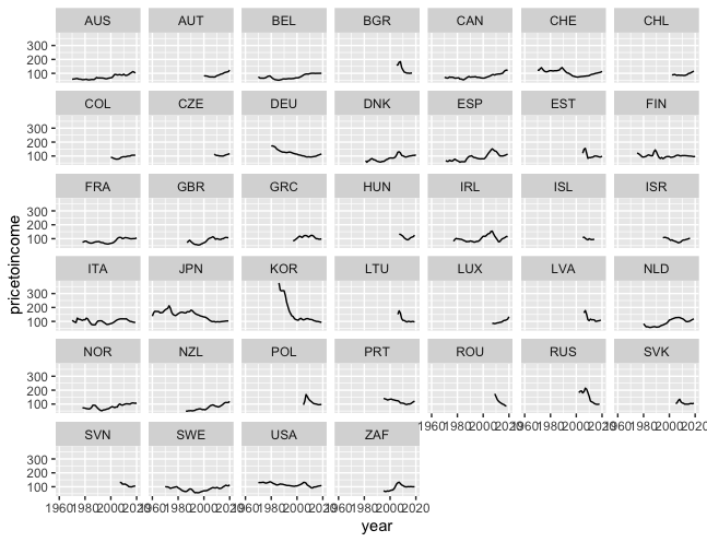
House Price to Income 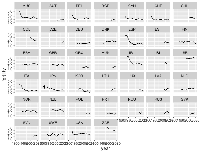
Fertility Rates
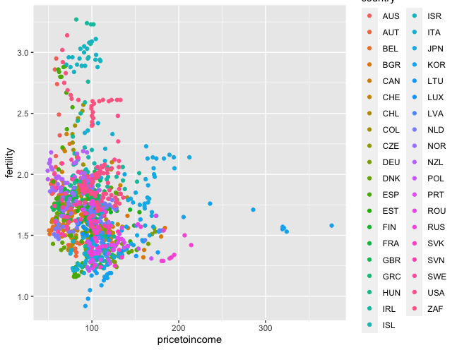
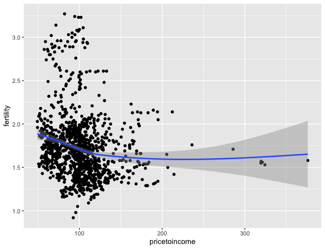
At a glance, I could not find a correlation between housing prices and fertility rates. So I changed the x and y axis to pricetoincome and fertility.
> ggplot(data=housing_fertility_df, aes(x = pricetoincome, y = fertility, color = country)) +
    geom_point()
> ggplot(data=housing_fertility_df, aes(x = pricetoincome, y = fertility)) +
    geom_point() +
    geom_smooth()
Maybe there is no correlation between house prices and fertility rates? I will now examine the relation between GDP per capita and fertility rates.
> gdpcap_fertility_df <- merge(oecd_gdp_cap, oecd_fertility_rates, by=c("country", "year"))
> ggplot(data=gdpcap_fertility_df, aes(x=gdpcap, y=fertility)) +
    geom_point()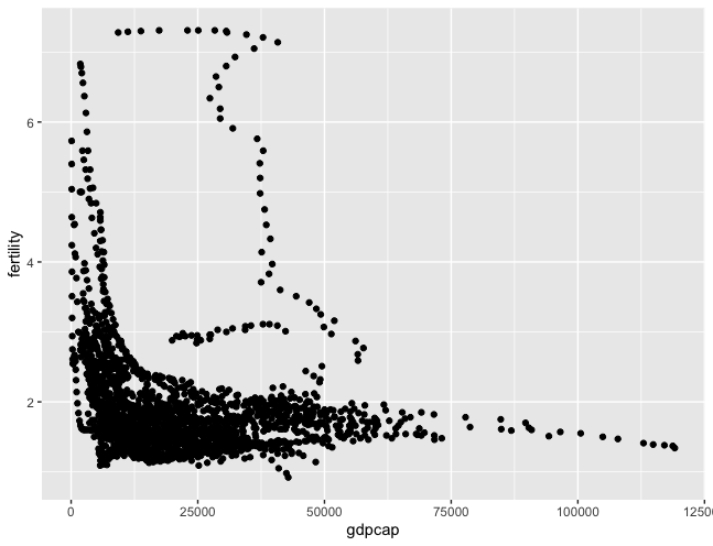
The graph is slightly representing an inverse relationship! Now I will add more layers.
> ggplot(data=gdpcap_fertility_df, aes(x=gdpcap, y=fertility)) +
    geom_point(aes(color=country)) +
    geom_smooth()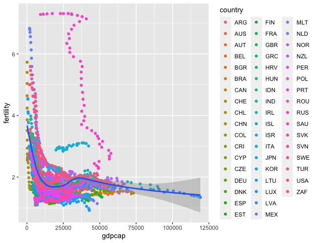
Now I want to look at the most recent data. I would like to to compare the GDP per capita from 2019.
> gdpcap_fertility_2019 <- filter(gdpcap_fertility_df, year==2019)
> ggplot(data=gdpcap_fertility_2019, aes(x=gdpcap, y=fertility)) +
+     geom_point(aes(color=country)) +
+     geom_smooth()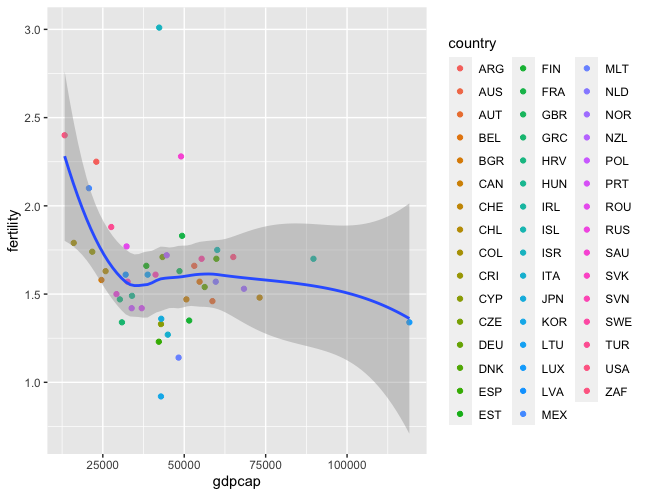
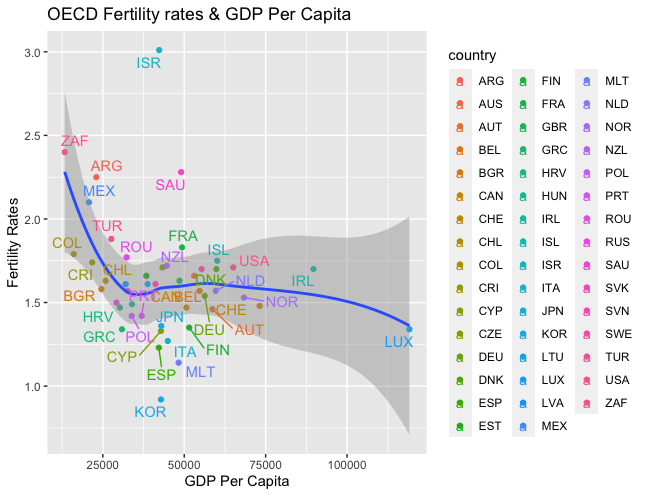
I can’t recognize the colors to the country names so I will add labels to the points. Additionally, I want to label the axises and display the title. But first, I need to install the ggrepel package first.
> install.packages("ggrepel")

> library(ggrepel)

> gf2019_df <- ggplot(data=gdpcap_fertility_2019, aes(x=gdpcap, y=fertility)) +
    geom_point(aes(color=country)) +
    geom_smooth() +
    geom_text_repel(aes(label=country, color=country))

> gf2019_df +
    labs(
         title = "OECD Fertility rates & GDP Per Capita",
         x = "GDP Per Capita",
         y = "Fertility Rates"
        )
4.2 What is the data telling us?
According to the analysis, there is no correlation between house prices to income and fertility rates. Rather, the correlation between GDP per capita and fertility rates resembled a negative relationship. One can rule that the overall income of individuals has greater effects on fertility rates, contrary to the belief that house prices are the driving force of decreasing fertility rates.
5. Act
A shrinking demographic may have negative effects on economic growth, while adding tax burdens to citizens. Many proponents of real estate regulation base their reasoning on decreasing fertility rates and acted accordingly to regulate the housing market, yet this neither achieved to decrease housing prices or increase fertility rates. According to the Federal Reserve Bank of St.Louis, the cause of lower fertility rates can be tracked down to education, hourly wages, infant mortality rates, and elderly care.
Therefore I propose the following to the legislative and executive branch of the Republic of Korea government:
- Provide affordable education. It is a known fact that education is crucial for higher wages. However, in this age where technology and knowledge evolves in an exponential rate, it is hard to say that a degree will guarantee a job. Rather, knowledge on a subject matter or highly desired skills can trump the value of what a degree can bring. While placing policies for affordable education, the content must be dynamic that it reflects the needs of the industry.
- Create high-paying jobs. While a well-educated population can create a workforce ready for sophisticated tasks, the market must be able to take on the supply. The government should incentivize startups and lure international corporations to enter the Korean market.
- Create sustainable daycare and elderly care systems. Families need time to take care of their children. But, in Korea when mothers and fathers sacrifice their time, more than often, they are paid back with the cold shoulder or at worse, nothing. The government should enforce paid parental leave proactively and contribute to build a culture where parents can spend time with their children.
